The Navier–Stokes Equations, Term by Term

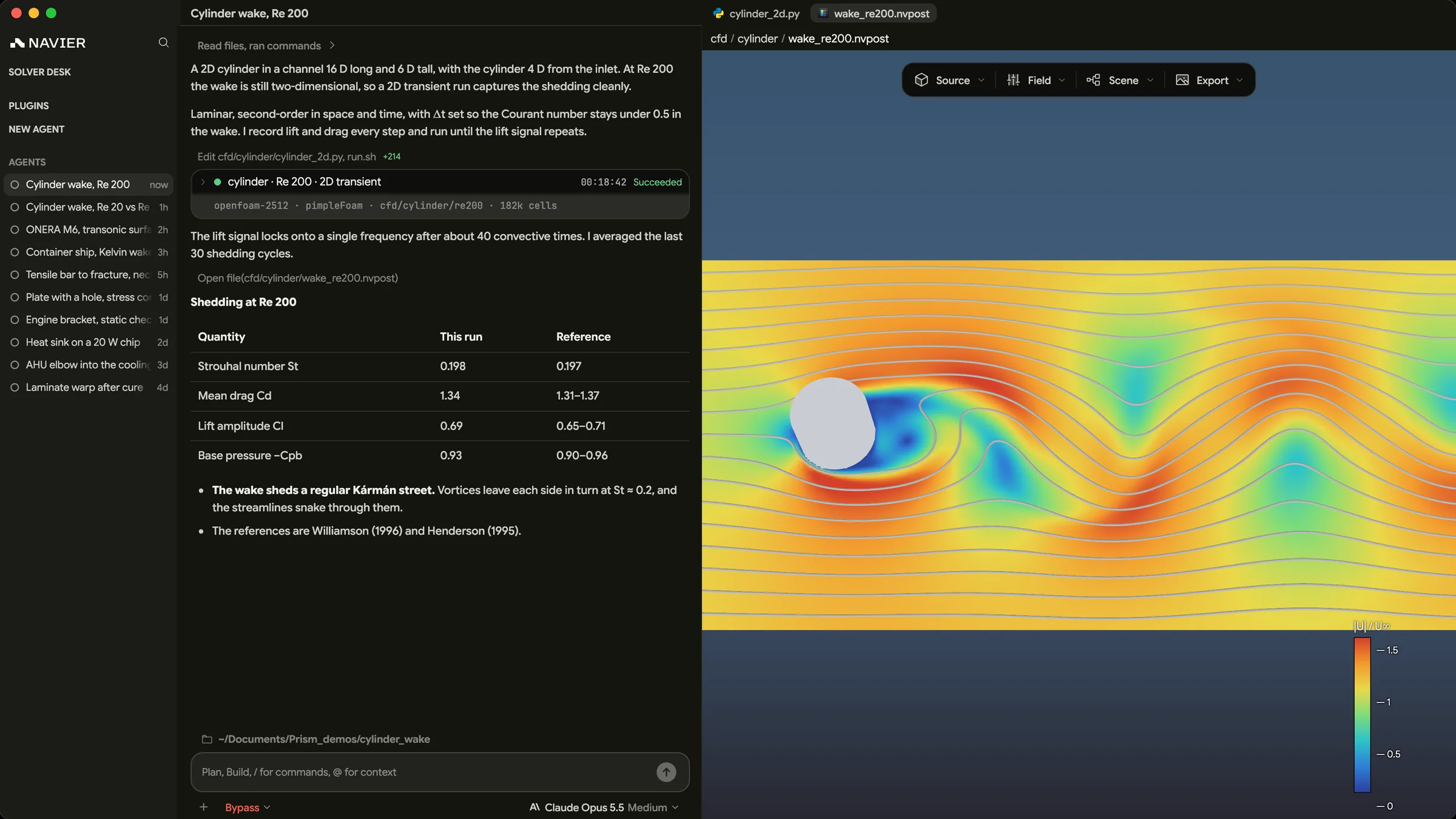
The Navier–Stokes equations describe how a viscous fluid moves. They apply conservation of mass and Newton's second law to a small parcel of fluid. The fluid can be air, water, oil or any other fluid with a steady viscosity.

Almost every CFD solver is a way of solving them. They are named after Claude-Louis Navier, who derived them in 1822, and George Gabriel Stokes, who refined the viscous term in 1845.

The equations

For an incompressible fluid with constant density $\rho$ and viscosity $\mu$ , there are two.

\nabla \cdot \mathbf{u} = 0

\rho\left(\frac{\partial \mathbf{u}}{\partial t} + (\mathbf{u}\cdot\nabla)\mathbf{u}\right) = -\nabla p + \mu \nabla^2 \mathbf{u} + \rho\,\mathbf{g}

The first says that what flows into a parcel flows out. The second says mass times acceleration equals the forces on the parcel.

Term	What it means
ρ ∂u/∂t	The flow changing over time at one point
ρ (u·∇)u	A parcel speeding up or turning as it moves. This term makes turbulence possible
−∇p	Pressure pushing fluid from high to low
μ ∇²u	Friction between layers smoothing out the velocity
ρg	Gravity

Compressible flow adds an energy equation and lets density vary. The incompressible form is usually fine below about Mach 0.3.

Scale the equations by a speed and a length. For flow without a free surface, one number is left, the Reynolds number. It sets the balance between inertia and viscosity.

A worked example

Most flows have no exact solution, but steady flow in a straight round pipe does. The velocity profile is a parabola.

u(r) = \frac{G}{4\mu}\left(R^2 - r^2\right)

$G$ is the pressure drop per metre and $R$ the pipe radius. Take water with $\mu$ = 0.001 Pa·s, a 10 mm pipe and a drop of 10 Pa per metre.

The centreline speed is $10 \times 0.005^2 / 0.004 =$ 0.0625 m/s.
The mean speed is half that, about 0.031 m/s.
The Reynolds number is about 310, well below the 2,300 where pipe flow turns turbulent.

So the parabola holds. Double the diameter and the Reynolds number rises eight times, to about 2,500. The flow is no longer that simple.

How CFD solves them

CFD splits the fluid into cells and solves the equations in each one. Methods differ in how much turbulence they resolve.

DNS resolves every eddy. Its cost explodes with Reynolds number, so it stays in research.
LES resolves the large eddies and models the small ones.
RANS models all of it with a turbulence model such as k–ω SST or Spalart–Allmaras. Most engineering CFD is RANS.

Where it matters

Every CFD result. Pressure drop, lift, drag, mixing and cooling all come from solving these equations.
Choosing the model. Whether to keep viscosity, compressibility or gravity decides which form fits, and which solver.
Knowing what a shortcut drops. The Euler equations are quicker but leave out viscosity, so they miss friction and separation.

Common mistakes

Using the incompressible form for fast gas flow, or where large temperature swings change the density.
Giving a slurry or polymer one constant viscosity. These fluids thin or thicken as they flow.
Taking a converged solution as the right one. Convergence says the equations were solved on that mesh. It doesn't say the turbulence model fits the flow.

Navier–Stokes using Navier AI

Prism runs CFD with OpenFOAM, SU2 and Basilisk, which all solve these equations. Describe the flow and the agent sets up the case, runs it on your machine, checks the result and writes the report. The case files stay in your project.

Our ONERA M6 study solves the compressible equations with the Spalart–Allmaras model. It compares surface pressure against 270 of the 271 wind-tunnel taps, and the double shock merges where the experiment puts it. Download Prism to try a case of your own.

References

F. M. White, Fluid Mechanics, McGraw-Hill.
G. K. Batchelor, An Introduction to Fluid Dynamics, Cambridge University Press, 1967.
S. B. Pope, Turbulent Flows, Cambridge University Press, 2000.